
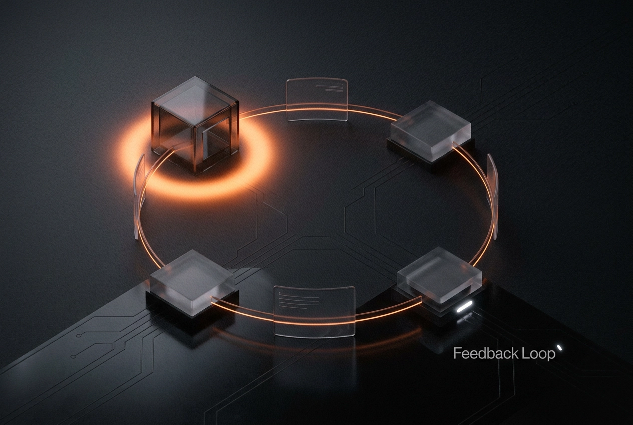
Every system that stays on track has something in common: it listens to itself. Your home thermostat does it. A jet engine does it. Even your body does it when it regulates your temperature. The secret ingredient holding all of it together is something called a feedback loop.
So what is the feedback loop definition, exactly? At its core, it is the mechanism by which a system measures its own output, compares that output to a target, and makes corrections to close the gap. Simple idea, enormous consequences.
If you are new to controls engineering, this is the single concept worth understanding before anything else. Once it clicks, everything that comes after, including PID controllers, PLCs, and SCADA systems, starts to make a lot more sense.
In this post, you will get a clear, jargon-free breakdown of how feedback loops work. You will see the idea come to life through a familiar thermostat example, learn the difference between negative and positive feedback, and understand why closed-loop systems outperform open-loop ones. By the end, you will have the foundation every other topic on this blog builds from.
Feedback Loop Definition: What It Actually Means
A feedback loop is the mechanism by which a system measures its own output, compares it to a desired target called the setpoint, and uses the difference to correct itself. Measure, compare, correct. That three-step cycle is the entire idea, and every control system you will ever work with runs on it.
To make that concrete, every feedback loop has four physical parts:
- Sensor – measures the actual output
- Comparator – calculates the difference between the measurement and the setpoint (that difference is called the error)
- Controller – decides what correction to apply based on the error
- Actuator – physically applies that correction to the process
Learn those four names now. You will see them in every example on this blog, from a home thermostat to a chemical reactor.
The word “feedback” itself describes signal direction. In a normal system, signals flow forward: command in, output out. In a feedback loop, the output signal travels backward through the system, back to the input, so the system can compare what actually happened against what was supposed to happen. That reverse path is the loop.
One important clarification: in controls engineering, “feedback loop” has a precise, hardware-grounded meaning. It is not a software pattern, a management concept, or a communication technique. It describes a physical circuit of measurement and correction.
That circuit is also the single unifying concept across every controls discipline. The same four-part loop structure runs a home thermostat, a cruise control system, a chemical reactor, and a jet engine turbine governor. The variables change; the loop does not. If you enjoy digging into that kind of systems thinking, Engineering For Fun: A Controls Engineer’s Blog by Atsu Bedjean is built exactly around it.
How a Thermostat Makes the Loop Concrete
Let’s put those four parts to work with an example you’ve lived with your whole life.
Set your thermostat to 70°F and here’s exactly what happens. The temperature sensor reads the actual room temperature, say 65°F, and reports it. The comparator subtracts that reading from your 70°F setpoint and gets a difference of 5°F. That difference is the error signal, and it’s the only thing driving the system forward. The controller sees a positive error and sends a “call for heat” signal. The furnace fires, which is the actuator doing its job.
Now the loop closes. The furnace pushes warm air into the room, the sensor detects the rising temperature, and the error signal shrinks. When the room hits 70°F, the error reaches zero. Zero error means no correction needed, so the furnace shuts off. No one touched the dial. The system regulated itself.
That’s the key insight: no error, no correction. The loop only acts when there’s a gap between where things are and where you want them to be.
This also explains why feedback control beats manual adjustment. A person guessing “it feels warm enough, I’ll turn off the heat” is reacting to a perception. The feedback loop reacts to a measurement. It responds to what’s actually happening, not what someone assumes is happening.
One more thing worth noting: the variable here is temperature, but the loop structure is identical for pressure, flow rate, speed, or position. Change the sensor and the actuator, and the same logic runs.
Negative Feedback Loops: The Stabilizing Force
The thermostat is a perfect first example, but notice something specific about how it works: every correction it makes opposes the deviation. Room too cold? The furnace pushes back. Room too warm? The cooling kicks in. That opposing relationship is the definition of negative feedback, and the word “negative” is purely a math term describing the sign of the correction, not a judgment about whether anything is going wrong.
Classic textbook examples make the pattern obvious:
- Cruise control on a car. You set 65 mph and hit a hill. Speed drops, the error signal grows, and the system opens the throttle wider to push back up to the setpoint. The correction opposes the drop.
- A pressure relief valve in a boiler. Pressure climbs past the safe limit, the valve opens and bleeds steam off until pressure falls back into range. Again, the correction fights the deviation.
- Blood glucose regulation. Blood sugar rises after a meal, your pancreas releases insulin to bring it back down. Same loop, different medium.
Negative feedback dominates engineering because it does three things reliably: it drives a system toward its setpoint, reduces steady-state error, and keeps behavior predictable even when conditions change.
The catch is that opposing every deviation too aggressively can cause a system to overshoot and oscillate, while reacting too slowly leaves it sluggish. Getting that balance right is exactly the problem that PID controllers solve, which is why they show up everywhere from industrial PLC loops to aircraft autopilots. The vast majority of intentionally designed control systems rely on negative feedback at their core, as any controls textbook will confirm.

Positive Feedback Loops: When Amplification Is the Point
Where negative feedback opposes deviation, positive feedback reinforces it, and things can escalate fast.
Common examples include a microphone held too close to a speaker. The mic picks up the speaker’s output, sends it back to the amplifier, which plays it louder, which the mic picks up again, louder still. Within fractions of a second you get that painful squeal. Each pass around the loop adds energy instead of subtracting it.
A more dangerous version happens in industrial settings. Imagine a steam boiler where a faulty inlet valve sticks open as pressure rises, allowing even more steam to build. Higher pressure, more inflow, higher pressure again. Without intervention, that loop ends at a physical limit, and not a pleasant one. In biology, population growth follows the same pattern: more individuals reproduce, producing more individuals, accelerating the growth rate further.
Positive feedback isn’t always a failure mode, though. Engineers deliberately build it into common applications such as oscillator circuits, Schmitt triggers, and latching relays. In those applications, you want a fast, decisive snap from one state to another, and positive feedback delivers exactly that. The loop races to a new stable state and locks there.
The contrast with negative feedback comes down to destination. Negative feedback seeks a setpoint and parks there. Positive feedback seeks a limit or a new state and sprints toward it.
Because unintended positive feedback can escalate a minor fault into a catastrophic one, it is one of the first failure modes engineers design against. Protective interlocks and safety systems exist specifically to break these runaway loops before they reach a destructive limit.
Open-Loop vs. Closed-Loop: Why Feedback Changes Everything
Both feedback types above share one thing: they exist inside a loop. But here’s a question worth asking first: what if there’s no loop at all?
Open-loop control means the system fires off a command and moves on, with no measurement of what actually happened. A toaster is the textbook example. You set the timer, it runs for that duration, and it stops. Burnt bread? Underdone bread? The toaster has no idea. It did its job as instructed, regardless of the result. A timer-based toaster works the same way whether or not the bread is actually done.
Closed-loop control is the opposite. The system continuously measures its output and adjusts in real time. A smart oven that monitors internal temperature and modulates the heating element to hit exactly 375°F is closed-loop. If opening the door drops the temperature, the oven responds immediately to recover it.
The practical tradeoff comes down to accuracy vs. simplicity:
- Open-loop: simpler, cheaper, no sensors or feedback controller required. But it drifts. Load changes, component wear, and environmental shifts will all pull the output away from the target, and the system has no way to notice or compensate.
- Closed-loop: self-correcting and far more accurate under real-world conditions. The added complexity and cost of sensors and controllers is the price of that reliability.
That said, open-loop is not the inferior choice by default. For well-understood, highly repeatable processes with minimal disturbances, it works fine and avoids unnecessary cost.
One last connection to close the loop (literally): a closed-loop system is simply a system that contains a feedback loop. The two terms describe the same architecture from different angles. “Closed-loop” refers to the circuit topology; “feedback loop” refers to the information flowing backward through it. Same thing.
The Control System Feedback Loop in Real Industrial Settings
The same four-part loop that governs your thermostat runs inside every industrial facility, just at much higher stakes. In a chemical plant flow control loop, a flow transmitter reads the pipe (sensor), a DCS or PLC calculates the error and decides on a correction (comparator and controller), and a control valve opens or closes to hit the target flow rate (actuator). Different hardware, same structure.
Industrial plants also layer loops inside each other. A common arrangement known as cascade control has an outer loop monitoring a slower variable, say temperature in a heat exchanger, with its output becoming the setpoint for a faster inner loop controlling flow. The inner loop reacts quickly enough to prevent disturbances from reaching the outer loop. This nesting is how plants achieve tight control over processes that would be impossible to manage with a single loop.
The hardware executing all of this is PLCs and DCS controllers, running the compare-and-correct cycle continuously. They never stop. In a typical industrial architecture, SCADA systems sit above the controller level, collecting data from every loop across the facility and displaying it to operators in a central interface. The loop runs in the PLC; operators see it in SCADA. (Dedicated posts on both are coming.)
One honest challenge worth flagging: sensors take a moment to respond, and control valves do not move instantly. That means the feedback loop is always acting on information that is slightly out of date. This built-in delay, called dead time, is one of the central problems in control loop tuning and a big reason why simple on/off control often falls short in industrial settings.
From Feedback Loops to PID: The Next Layer of Precision
That on/off behavior, bang-bang control, produces the sawtooth oscillation you saw in the thermostat example. That behavior has a name: bang-bang control. It works, but it never actually settles.
PID control solves this by making the correction proportional to the situation. Instead of flipping a switch, a PID controller reads the error signal in three ways simultaneously:
- Proportional (P): reacts to the current error. Bigger error, stronger correction.
- Integral (I): accumulates past error over time and corrects for persistent drift that P alone misses.
- Derivative (D): watches the rate of change and applies a braking force before the output overshoots.
Together, the three terms produce corrections that are smooth, fast, and accurate rather than blunt.
PID is widely regarded as one of the most commonly deployed control strategies in engineering practice, and a big reason is that it handles real-world variation well even without a precise mathematical model of the process being controlled.
One thing worth stressing: PID does not replace the feedback loop. The four-part structure, sensor, comparator, controller, actuator, stays exactly the same. PID simply makes the controller block smarter. The loop is the architecture; PID is the logic running inside it.
That distinction is the bridge to the next topic. Once the loop structure is solid in your mind, PID tuning stops feeling abstract and starts making intuitive sense. The deep dive is up next in the PID post.
One Idea, Every Control System
Every control system, from a home thermostat to a full industrial automation stack, runs on the same four-step loop. That’s the whole idea, and everything else in controls engineering is just a variation on it.
A few distinctions are worth keeping straight as you move forward:

- Negative vs. positive feedback: Negative feedback stabilizes (see above); positive feedback amplifies.
- Open-loop vs. closed-loop: Open-loop applies a fixed output; closed-loop self-corrects through the feedback loop.
- On/off control vs. PID: Bang-bang control causes oscillation; PID adds proportional, integral, and derivative logic for smoother corrections within the same loop structure.
Here’s a habit worth building right now: the next time you interact with any automatically controlled system, a car’s cruise control, an HVAC unit, a conveyor line, pause and identify the four parts. What’s the sensor? Where does the comparison happen? What’s the controller doing? What’s the actuator? You’ll start seeing the loop everywhere, and each time you spot it, your intuition gets a little sharper.
This foundation is genuinely leveraged learning. The time you invest in understanding feedback loops pays dividends across every controls topic you encounter next. PID tuning clicks faster when the loop structure is already clear. PLC programming makes more sense when you recognize the compare-and-correct logic behind every rung. SCADA becomes readable when you understand what those loops are actually doing at the field level.
Each of those topics builds directly on what you’ve learned here, and dedicated posts on each one are coming up next on the blog.
Conclusion
Feedback loops are the foundational idea behind every control system you will ever work with. As covered above, the four-part loop structure, the distinction between negative and positive feedback, the difference between open- and closed-loop architectures, and PID’s role as a precision layer on top of that structure are the core ideas that unlock everything else in controls engineering.
Your next step is simple: pick one system around you today and map its four parts. The loop is already there. You just have to look.
Everything you encounter next in controls, whether PID tuning, PLC logic, or SCADA systems, grows from this single idea. You have already built the mental model that makes all of it learnable. Keep going.
Frequently Asked Questions
What are the four main components of a feedback loop?
Every feedback loop consists of four physical parts: (1) Sensor – measures the actual output, (2) Comparator – calculates the difference between the measurement and the setpoint (called the error), (3) Controller – decides what correction to apply based on the error, and (4) Actuator – physically applies that correction to the process. These four components work together in a continuous cycle of measure, compare, and correct.
What's the difference between negative and positive feedback loops?
Negative feedback loops oppose deviations to stabilize a system toward its setpoint. For example, a thermostat heating when it's cold or cooling when it's warm. Negative feedback reduces error and keeps behavior predictable. Positive feedback, by contrast, reinforces deviations and amplifies changes. A microphone creating feedback near a speaker is a classic example. While positive feedback can cause runaway conditions, it's sometimes deliberately used in applications like oscillator circuits for fast, decisive state changes.
Why is closed-loop control better than open-loop control?
Closed-loop systems continuously measure output and adjust in real time, making them self-correcting and far more accurate under real-world conditions. Open-loop systems apply a fixed command without feedback, like a timer-based toaster. However, closed-loop systems require additional sensors and controllers, adding complexity and cost. Open-loop is simpler and cheaper for well-understood, highly repeatable processes with minimal disturbances. The choice depends on balancing accuracy against simplicity and cost.
How does a home thermostat use feedback loops to regulate temperature?
A thermostat demonstrates the feedback loop perfectly: the temperature sensor reads the actual room temperature and compares it to your setpoint (say 70°F). The comparator calculates the error (difference). If the room is 65°F, the error is 5°F, which tells the controller to signal the furnace to turn on. As the room warms, the error shrinks. When the room reaches exactly 70°F, the error becomes zero, and the furnace shuts off automatically. The system regulates itself without any further manual adjustment.
What is dead time in a feedback loop, and why does it matter?
Dead time is the built-in delay that occurs because sensors take time to respond and actuators (like control valves) don't move instantly. This means feedback loops are always acting on information that is slightly out of date. Dead time is one of the central problems in control loop tuning and a key reason why simple on/off (bang-bang) control often falls short in industrial settings. Understanding and accounting for dead time is critical when designing effective control systems.
Leave a Reply